张量
类似 Numpy 中的 ndarray, 区别在于能够利用 GPU 进行并行计算.
初始化
有多种初始化张量的方法,示例如下:
1
2
3
4
5
6
7
8
9
10
11
12
13
14
15
16
17
import torchimport numpy as np1 , 2 ], [3 , 4 ]]print (f"Ones Tensor: \n {x_ones} \n" )float ) print (f"Random Tensor: \n {x_rand} \n" )
1
2
3
4
5
6
7
Ones Tensor:
张量属性
形状, 数据类型, 存储设备
1
2
3
4
5
tensor = torch.rand(3 , 4 )print (f"Shape of tensor: {tensor.shape} " )print (f"Datatype of tensor: {tensor.dtype} " )print (f"Device tensor is stored on: {tensor.device} " )
1
2
3
Shape of tensor: torch.Size([3, 4])
张量操作
张量支持非常多的操作, 100 多种,例如转置, 索引, 切片, 数学去处, 线性代数, 随机抽样等等.
可将张量移动到 GPU 进行计算, 可以显著提高计算的速度.
1 2 3 4 if torch.cuda.is_available():'cuda' )print (f"Device tensor is stored on: {tensor.device} " )
1 Device tensor is stored on: cuda:0
类似 Numpy 的索引和切片
1
2
3
tensor = torch.ones(4 , 4 )1 ] = 0 print (tensor)
1
2
3
4
tensor([[1., 0., 1., 1.],
归并 concate
1
2
t1 = torch.cat([tensor, tensor, tensor], dim=1 )print (t1)
1
2
3
4
tensor([[1., 0., 1., 1., 1., 0., 1., 1., 1., 0., 1., 1.],
逐元素乘法
1 2 3 4 5 6 7 8 1 , 2 ], [3 , 4 ]])5 , 6 ], [7 , 8 ]])
1 2 3 4 5 6 7 8 1 , 2 ], [3 , 4 ]]) 10 , 20 ])
矩阵乘法
torch.matmul() 或者使用运算符 @
1
2
3
4
5
6
7
a = torch.tensor([[1 , 2 ], [3 , 4 ]]) 5 , 6 ], [7 , 8 ]])
计算过程:
第一行第一列:1×5 + 2×7 = 19
就地更新
在原方法的末尾添加下划线即可
1
2
3
print (tensor, "\n" )5 ) print (tensor)
1
2
3
4
5
6
7
8
9
tensor([[1., 0., 1., 1.],
关联 Numpy
在 CPU 上的张量可以和 Numpy 共享内存, 修改其中一个会直接影响另外一个
张量转 Numpy 数组
1
2
3
4
t = torch.ones(5 )print (f"t: {t} " )print (f"n: {n} " )
1
2
t: tensor([1., 1., 1., 1., 1.])
当修改张量后, numpy 数组也会跟着变化
1 2 3 t.add_(1 )print (f"t: {t} " )print (f"n: {n} " )
1
2
t: tensor([2., 2., 2., 2., 2.])
Numpy数组转张量
修改 numpy 数组也会让张量跟着变化
1
2
n = np.ones(5 )
1
2
3
np.add(n, 1, out=n) print (f"t: {t}" )print (f"n: {n}" )
1
2
t: tensor([2., 2., 2., 2., 2.], dtype=torch.float64)
自动梯度
1
2
3
4
5
6
7
8
9
10
11
12
13
14
15
import torchfrom torchvision.models import resnet18, ResNet18_Weights1 , 3 , 64 , 64 )1 , 1000 )sum ()1e-2 , momentum=0.9 )
自动计算梯度的示例
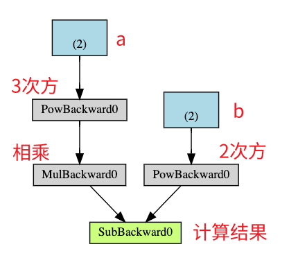
1
2
3
4
import torch2. , 3. ], requires_grad=True )6. , 4. ], requires_grad=True )
假设:
Q = 3 a 3 − b 2
假设 a、b 为权重参数,那么 Q 相对 a,b 的导数为:
∂ Q ∂ a = 9 a 2
∂ Q ∂ b = − 2 b
1 2 3 1. , 1. ])
1
2
3
4
print (9 *a**2 == a.grad)print (-2 *b == b.grad)print (a.grad)print (b.grad)
1
2
3
4
tensor([True, True])
导数的本质是变化率,即当自变量 x 出现 1 个单位的变化时, 因变量 y 会出现多大的变化. 而损失值则是期待的变化幅度(变了多少个单位后将满足目标值).
计算图
当调用 loss.backward() 时, torch 会自动计算损失向量(梯度)的雅可比积, 将损失函数的梯度反向传播到所有相关的可训练权重参数, 用于后续的参数更新. 损失值与梯度的乘积即表示参数应该更新的量, 但通常会乘以一个学习率,以便实现小幅度的更新, 避免过于剧烈的震荡.
计算图是一个单向无环图(DAG), 记录着从输入的张量到输出的张量之间的每一步计算过程.
计算图是在前向传播的过程中动态构建的, 同时在调用 backward() 方法后会自动释放, 以便节省内存. 如果缓存计算图, 需要设置参数 retain_graph=true. 当重复调用 backward 时, 会报错. 因为第一次调用后会释放, 导致后续的调用找不到计算图了.
如果某个张量不需要构建计算图, 可设置参数 required_grad=False
1
2
3
4
5
6
7
8
x = torch.rand(5 , 5 )5 , 5 )5 , 5 ), requires_grad=True )print (f"Does `a` require gradients?: {a.requires_grad} " )print (f"Does `b` require gradients?: {b.requires_grad} " )
1
2
Does `a` require gradients?: False
当设置 required_grad=False 时, 因为没有构建计算图, 因此参数在训练过程中不会被更新, 相当于被冻结了. 这个功能在微调模型的场景中很有用, 因为我们通常需要冻结主干模型, 只训练最后的分类层.
1
2
3
4
5
6
7
8
9
10
11
12
13
from torch import nn, optimfor param in model.parameters():False 512 , 10 )1e-2 , momentum=0.9 )
另外还有一个全局的暂停自动梯度计算的方法是使用 torch.no_grad()
神经网络
nn.Module 类可用来构建一个神经网络中的模块(神经元), 模块由一个或多个层构成, 有一个 forward 前向传播的方法, 并返回一个计算结果 output
神经元通常包含一个非线性的激活层, 以便能够实现对复杂函数的拟合.
网络示例
1
2
3
4
5
6
7
8
9
10
11
12
13
14
15
16
17
18
19
20
21
22
23
24
25
26
27
28
29
30
31
32
33
34
35
36
37
38
39
40
41
42
43
44
45
46
47
import torchimport torch.nn as nnimport torch.nn.functional as Fclass Net (nn.Module):def __init__ (self ):super (Net, self ).__init__()self .conv1 = nn.Conv2d(1 , 6 , 5 )self .conv2 = nn.Conv2d(6 , 16 , 5 )self .fc1 = nn.Linear(16 * 5 * 5 , 120 ) self .fc2 = nn.Linear(120 , 84 )self .fc3 = nn.Linear(84 , 10 )def forward (self, input ):self .conv1(input ))2 , 2 ))self .conv2(s2))2 )1 )self .fc1(s4))self .fc2(f5))self .fc3(f6)return outputprint (net)
1
2
3
4
5
6
7
Net(
可使用 model.parameters() 方法访问所有可学习参数
1
2
3
params = list (net.parameters())print (len (params))print (params[0 ].size())
1
2
10
可使用 model.zero_grad() 方法重置梯度
1 2 net.zero_grad()1 , 10 ))
torch.nn 强制要求样本以批次为单位作为输入, 不能以单个样本为单位作为输入. 最小批次数量为 1, 因此输入张量的第 1 个维度即是单批的样本数量. 如果每批只有一个样本, 则该值为 1.
对于单个样本, 可使用 input.unsqueeze(0) 方法, 给样本添加一个批次的维度
损失函数
损失函数用于计算模型的输出和目标值之间的差异
1
2
3
4
5
6
7
output = net(input )10 ) 1 , -1 ) print (loss)
1 tensor(1.2850, grad_fn=<MseLossBackward0>)
以下是损失张量的计算图
1
2
3
4
input -> conv2d -> relu -> maxpool2d -> conv2d -> relu -> maxpool2d
1
2
3
print (loss.grad_fn) print (loss.grad_fn.next_functions[0 ][0 ]) print (loss.grad_fn.next_functions[0 ][0 ].next_functions[0 ][0 ])
1
2
3
<MseLossBackward0 object at 0x7febcb77eb00>
反向传播
梯度值是累加的, 因此每次进行反向传播时, 需要先调用 model.zero_grad 方法重置梯度值
1
2
3
4
5
6
7
8
9
net.zero_grad() print ('conv1.bias.grad before backward' )print (net.conv1.bias.grad)print ('conv1.bias.grad after backward' )print (net.conv1.bias.grad)
1
2
3
4
conv1.bias.grad before backward
更新参数
对于 SGD 小批量梯度优化器, 参数的更新规则如下:
1 weight = weight - learning_rate * gradient
使用 python 代码实现如下:
1
2
3
learning_rate = 0.01 for f in net.parameters():
除了 SGD 外, 还有很多种参数更新方法, 例如: Nesterov-SGD, Adam, RMSProp 等. 可以使用 torch.optim 进行初始化, 选择合适的优化器, 实现对参数的更新
1
2
3
4
5
6
7
8
9
10
11
import torch.optim as optim0.01 )input )
训练分类器
数据预处理
可使用一些常见的 python 库将文本, 图片, 音频, 视频等数据转成 numpy 格式, 然后再转成 Tensor 张量. 对于视频类型的数据, torch 有一个专门的 torchvision 库可实现常见数据集的加载和预处理.
训练图片分类器
加载数据并规范化
此处以 CIFAR10 数据集进行示例
1
2
3
import torchimport torchvisionimport torchvision.transforms as transforms
1
2
3
4
5
6
7
8
9
10
11
12
13
14
15
16
17
18
19
transform = transforms.Compose(0.5 , 0.5 , 0.5 ), (0.5 , 0.5 , 0.5 ))]) 4 './data' , train=True ,True , transform=transform)True , num_workers=2 )'./data' , train=False ,True , transform=transform)False , num_workers=2 )'plane' , 'car' , 'bird' , 'cat' ,'deer' , 'dog' , 'frog' , 'horse' , 'ship' , 'truck' )
定义神经网络
1
2
3
4
5
6
7
8
9
10
11
12
13
14
15
16
17
18
19
20
21
22
23
24
25
import torch.nn as nnimport torch.nn.functional as Fclass Net (nn.Module):def __init__ (self ):super ().__init__()self .conv1 = nn.Conv2d(3 , 6 , 5 )self .pool = nn.MaxPool2d(2 , 2 )self .conv2 = nn.Conv2d(6 , 16 , 5 )self .fc1 = nn.Linear(16 * 5 * 5 , 120 )self .fc2 = nn.Linear(120 , 84 )self .fc3 = nn.Linear(84 , 10 )def forward (self, x ):self .pool(F.relu(self .conv1(x)))self .pool(F.relu(self .conv2(x)))1 ) self .fc1(x))self .fc2(x))self .fc3(x)return x
定义损失函数和优化器
1
2
3
4
import torch.optim as optim0.001 , momentum=0.9 )
训练网络
1
2
3
4
5
6
7
8
9
10
11
12
13
14
15
16
17
18
19
20
21
22
23
for epoch in range (2 ): 0.0 for i, data in enumerate (trainloader, 0 ):if i % 2000 == 1999 : print (f'[{epoch + 1 } , {i + 1 :5d} ] loss: {running_loss / 2000 :.3 f} ' )0.0 print ('Finished Training' )
1
2
3
4
5
6
7
8
9
10
11
12
13
[1, 2000] loss: 2.229
保存训练后的模型参数
1
2
PATH = './cifar_net.pth'
测试网络模型
1
2
3
4
5
dataiter = iter (testloader)next (dataiter)True ))
1
2
3
4
5
6
outputs = net(images)max (outputs, 1 )print ('Predicted: ' , ' ' .join(f'{classes[predicted[j]]:5s} ' for j in range (4 )))
1 Predicted: cat ship ship ship
使用 GPU 训练
1
2
3
4
5
device = torch.device('cuda:0' if torch.cuda.is_available() else 'cpu' )0 ].to(device), data[1 ].to(device)
多 GPU 训练
1 2 3 4 5 6 7 "cuda:0" )
准备数据
1
2
3
4
5
6
7
8
9
10
import torchimport torch.nn as nnfrom torch.utils.data import Dataset, DataLoader5 2 30 100
1 device = torch.device("cuda:0" if torch.cuda.is_available() else "cpu" )
1 2 3 4 5 6 7 8 9 10 11 12 13 14 15 class RandomDataset (Dataset ):def __init__ (self, size, length ):self .len = lengthself .data = torch.randn(length, size)def __getitem__ (self, index ):return self .data[index]def __len__ (self ):return self .len True )
准备模型
1
2
3
4
5
6
7
8
9
10
11
12
13
class Model (nn.Module):def __init__ (self, input_size, output_size ):super (Model, self ).__init__()self .fc = nn.Linear(input_size, output_size)def forward (self, input ):self .fc(input )print ("\tIn Model: input size" , input .size(),"output size" , output.size())return output
并行训练
检查是否有多个 GPU 可用, 如有, 开启并行训练
1
2
3
4
5
6
7
model = Model(input_size, output_size)if torch.cuda.device_count() > 1 :print ("Let's use" , torch.cuda.device_count(), "GPUs!" )
1 2 3 4 5 6 7 Let's use 4 GPUs! DataParallel( (module): Model( (fc): Linear(in_features=5, out_features=2, bias=True) ) )
运行模型
1
2
3
4
5
for data in rand_loader:input = data.to(device)input )print ("Outside: input size" , input .size(),"output_size" , output.size())
以下是有 4 个 GPU 并行时的输出
1
2
3
4
5
6
7
8
9
10
11
12
13
14
15
16
Outside: input size torch.Size([30, 5]) output_size torch.Size([30, 2])
2 个 GPU 时:
1 2 3 4 5 6 7 8 9 10 11 12 13 14 's use 2 GPUs! In Model: input size torch.Size([15, 5]) output size torch.Size([15, 2]) In Model: input size torch.Size([15, 5]) output size torch.Size([15, 2]) Outside: input size torch.Size([30, 5]) output_size torch.Size([30, 2]) In Model: input size torch.Size([15, 5]) output size torch.Size([15, 2]) In Model: input size torch.Size([15, 5]) output size torch.Size([15, 2]) Outside: input size torch.Size([30, 5]) output_size torch.Size([30, 2]) In Model: input size torch.Size([15, 5]) output size torch.Size([15, 2]) In Model: input size torch.Size([15, 5]) output size torch.Size([15, 2]) Outside: input size torch.Size([30, 5]) output_size torch.Size([30, 2]) In Model: input size torch.Size([5, 5]) output size torch.Size([5, 2]) In Model: input size torch.Size([5, 5]) output size torch.Size([5, 2]) Outside: input size torch.Size([10, 5]) output_size torch.Size([10, 2])
3 个 GPU 时
1 2 3 4 5 6 7 8 9 10 11 12 13 14 15 16 17 Let's use 3 GPUs! In Model: input size torch.Size([10, 5]) output size torch.Size([10, 2]) In Model: input size torch.Size([10, 5]) output size torch.Size([10, 2]) In Model: input size torch.Size([10, 5]) output size torch.Size([10, 2]) Outside: input size torch.Size([30, 5]) output_size torch.Size([30, 2]) In Model: input size torch.Size([10, 5]) output size torch.Size([10, 2]) In Model: input size torch.Size([10, 5]) output size torch.Size([10, 2]) In Model: input size torch.Size([10, 5]) output size torch.Size([10, 2]) Outside: input size torch.Size([30, 5]) output_size torch.Size([30, 2]) In Model: input size torch.Size([10, 5]) output size torch.Size([10, 2]) In Model: input size torch.Size([10, 5]) output size torch.Size([10, 2]) In Model: input size torch.Size([10, 5]) output size torch.Size([10, 2]) Outside: input size torch.Size([30, 5]) output_size torch.Size([30, 2]) In Model: input size torch.Size([4, 5]) output size torch.Size([4, 2]) In Model: input size torch.Size([4, 5]) output size torch.Size([4, 2]) In Model: input size torch.Size([2, 5]) output size torch.Size([2, 2]) Outside: input size torch.Size([10, 5]) output_size torch.Size([10, 2])
8 个 GPU 时
1 2 3 4 5 6 7 8 9 10 11 12 13 14 15 16 17 18 19 20 21 22 23 24 25 26 27 28 29 30 31 32 33 34 Let's use 8 GPUs! In Model: input size torch.Size([4, 5]) output size torch.Size([4, 2]) In Model: input size torch.Size([4, 5]) output size torch.Size([4, 2]) In Model: input size torch.Size([2, 5]) output size torch.Size([2, 2]) In Model: input size torch.Size([4, 5]) output size torch.Size([4, 2]) In Model: input size torch.Size([4, 5]) output size torch.Size([4, 2]) In Model: input size torch.Size([4, 5]) output size torch.Size([4, 2]) In Model: input size torch.Size([4, 5]) output size torch.Size([4, 2]) In Model: input size torch.Size([4, 5]) output size torch.Size([4, 2]) Outside: input size torch.Size([30, 5]) output_size torch.Size([30, 2]) In Model: input size torch.Size([4, 5]) output size torch.Size([4, 2]) In Model: input size torch.Size([4, 5]) output size torch.Size([4, 2]) In Model: input size torch.Size([4, 5]) output size torch.Size([4, 2]) In Model: input size torch.Size([4, 5]) output size torch.Size([4, 2]) In Model: input size torch.Size([4, 5]) output size torch.Size([4, 2]) In Model: input size torch.Size([4, 5]) output size torch.Size([4, 2]) In Model: input size torch.Size([2, 5]) output size torch.Size([2, 2]) In Model: input size torch.Size([4, 5]) output size torch.Size([4, 2]) Outside: input size torch.Size([30, 5]) output_size torch.Size([30, 2]) In Model: input size torch.Size([4, 5]) output size torch.Size([4, 2]) In Model: input size torch.Size([4, 5]) output size torch.Size([4, 2]) In Model: input size torch.Size([4, 5]) output size torch.Size([4, 2]) In Model: input size torch.Size([4, 5]) output size torch.Size([4, 2]) In Model: input size torch.Size([4, 5]) output size torch.Size([4, 2]) In Model: input size torch.Size([4, 5]) output size torch.Size([4, 2]) In Model: input size torch.Size([4, 5]) output size torch.Size([4, 2]) In Model: input size torch.Size([2, 5]) output size torch.Size([2, 2]) Outside: input size torch.Size([30, 5]) output_size torch.Size([30, 2]) In Model: input size torch.Size([2, 5]) output size torch.Size([2, 2]) In Model: input size torch.Size([2, 5]) output size torch.Size([2, 2]) In Model: input size torch.Size([2, 5]) output size torch.Size([2, 2]) In Model: input size torch.Size([2, 5]) output size torch.Size([2, 2]) In Model: input size torch.Size([2, 5]) output size torch.Size([2, 2]) Outside: input size torch.Size([10, 5]) output_size torch.Size([10, 2])
DataParallel 实现的是数据并行, 即将数据拆分到不同的 GPU 上进行计算, 最后再合并计算结果.
简单示例
numpy
使用 numpy 来计算梯度的示例
1 2 3 4 5 6 7 8 9 10 11 12 13 14 15 16 17 18 19 20 21 22 23 24 25 26 27 28 29 30 31 32 33 34 35 36 37 38 import numpy as npimport math2000 )1e-6 for t in range (2000 ):2 + d * x ** 3 sum ()if t % 100 == 99 :print (t, loss)2.0 * (y_pred - y) sum () sum ()2 ).sum ()3 ).sum ()print (f'Result: y = {a} + {b} x + {c} x^2 + {d} x^3' )
由于损失值的计算公式如下:
L = ∑ ( y ^ − y ) 2 , y ^ = a + b x + c x 2 + d x 3
因此, 损失 L 相对 a, b, c, d 的导数计算公式如下:
∂ L ∂ a = ∑ 2 ( y ^ − y ) ⋅ 1 = grad_a
∂ L ∂ b = ∑ 2 ( y ^ − y ) ⋅ x = grad_b
∂ L ∂ c = ∑ 2 ( y ^ − y ) ⋅ x 2 = grad_c
∂ L ∂ d = ∑ 2 ( y ^ − y ) ⋅ x 3 = grad_d
Tensors
相比 numpy array, Tensor 最大的好处是可以利用 GPU 实现并行计算, 能够显著提高计算速度(可能达50x)
1 2 3 4 5 6 7 8 9 10 11 12 13 14 15 16 17 18 19 20 21 22 23 24 25 26 27 28 29 30 31 32 33 34 35 36 37 38 39 40 41 42 43 44 import torchimport mathfloat "cpu" ) 2000 , device=device, dtype=dtype)1e-6 for t in range (2000 ):2 + d * x ** 3 pow (2 ).sum ().item()if t % 100 == 99 :print (t, loss)2.0 * (y_pred - y)sum ()sum ()2 ).sum ()3 ).sum ()print (f'Result: y = {a.item()} + {b.item()} x + {c.item()} x^2 + {d.item()} x^3' )
Autograd
以上示例是手动实现前向和反向传播, 对于只有1~2 层的神经网络来说还可以接受. 但对于深度神经网络来说, 工作量就会变得非常恐怖了. PyTorch 通过引入计算图, 来实现自动的梯度计算.
计算图的节点是输入张量, 边是计算输出张量的函数. 例如假设 x 是一个输入张量, 那么 x.grad 里面将用于存放输出的标量相对于 x 的梯度.
1
2
3
4
5
6
7
8
9
10
11
12
13
14
15
16
17
18
19
20
21
22
23
24
25
26
27
28
29
30
31
32
33
34
35
36
37
38
39
40
41
42
43
44
45
46
47
48
import torchimport mathfloat type if torch.accelerator.is_available() else "cpu" print (f"Using {device} device" )1 , 1 , 2000 , dtype=dtype)True )True )True )True )1. 1e-5 for t in range (5000 ):2 + d * x ** 3 pow (2 ).sum ()if t==0 :if t % 100 == 99 :print (f'Iteration t = {t:4d} loss(t)/loss(0) = {round (loss.item()/initial_loss, 6 ):10.6 f} a = {a.item():10.6 f} b = {b.item():10.6 f} c = {c.item():10.6 f} d = {d.item():10.6 f} ' )with torch.no_grad():None None None None print (f'Result: y = {a.item()} + {b.item()} x + {c.item()} x^2 + {d.item()} x^3' )
自定义 autograd
autograd 运算符实际由两个函数构成,一个是前向传播函数, 它根据输入计算输出. 一个是反向传播函数, 它根据输出张量相某个标量损失的梯度计算输入张量相对同一个标量损失的梯度.
通过继承 torch.autograd.Function 可以自定义 autograd 运算符, 只需实现 forward 和 backward 函数即可.
1
2
3
4
5
6
7
8
9
10
11
12
13
14
15
16
17
18
19
20
21
22
23
24
25
26
27
28
29
30
31
32
33
34
35
36
37
38
39
40
41
42
43
44
45
46
47
48
49
50
51
52
53
54
55
56
57
58
59
60
61
62
63
64
65
import torchimport mathclass LegendrePolynomial3 (torch.autograd.Function):""" 通过继承 torch.autograd.Function 类,并实现其中的前向传播和反向传播方法来创建自定义的自动求导函数。这些方法操作的是张量 """ @staticmethod def forward (ctx, input ):""" 在前向传播中,会接收到一个包含输入数据的张量,并返回一个包含输出结果的张量。ctx是一个上下文对象,可用于暂存反向传播计算所需的信息。可以通过 ctx.save_for_backward方法缓存张量以供反向传播使用。其他对象可以直接作为 ctx对象的属性存储,例如 ctx.my_object = my_object """ input )return 0.5 * (5 * input ** 3 - 3 * input ) @staticmethod def backward (ctx, grad_output ):""" 在反向传播中,会接收到一个包含损失相对于输出梯度的张量,然后需要计算损失相对于输入的梯度。 """ input , = ctx.saved_tensorsreturn grad_output * 1.5 * (5 * input ** 2 - 1 )float "cpu" )2000 , device=device, dtype=dtype)0.0 , device=device, dtype=dtype, requires_grad=True )1.0 , device=device, dtype=dtype, requires_grad=True )0.0 , device=device, dtype=dtype, requires_grad=True )0.3 , device=device, dtype=dtype, requires_grad=True )5e-6 for t in range (2000 ):pow (2 ).sum ()if t % 100 == 99 :print (t, loss.item())with torch.no_grad():None None None None print (f'Result: y = {a.item()} + {b.item()} * P3({c.item()} + {d.item()} x)' )
nn 模块
相比 autograd 运算符, nn.Module 提供了一个更高层级的抽象, 以便能够更加便捷的构建神经网络, 它有点类似于网络中的层.
nn 库中包括一些模块(Modules) 同样是基于输入张量, 计算输出张量. 但它拥有一些内部状态, 例如包含可学习参数. nn 库还包含一些常用的损失函数.
1 2 3 4 5 6 7 8 9 10 11 12 13 14 15 16 17 18 19 20 21 22 23 24 25 26 27 28 29 30 31 32 33 34 35 36 37 38 39 40 41 42 43 44 45 46 47 48 49 50 51 52 import torchimport math2000 )1 , 2 , 3 ])1 )pow (p) 3 , 1 ),0 , 1 )'sum' )1e-6 for t in range (2000 ):if t % 100 == 99 :print (t, loss.item())with torch.no_grad():for param in model.parameters():0 ]print (f'Result: y = {linear_layer.bias.item()} + {linear_layer.weight[:, 0 ].item()} x + {linear_layer.weight[:, 1 ].item()} x^2 + {linear_layer.weight[:, 2 ].item()} x^3' )
optim
nn 库使用 optim 类实现对参数优化算法的封装
1 2 3 4 5 6 7 8 9 10 11 12 13 14 15 16 17 18 19 20 21 22 23 24 25 26 27 28 29 30 31 32 33 import torchimport math2000 )1 , 2 , 3 ])1 ).pow (p)3 , 1 ),0 , 1 )'sum' )1e-3 for t in range (2000 ):if t % 100 == 99 :print (t, loss.item())0 ]print (f'Result: y = {linear_layer.bias.item()} + {linear_layer.weight[:, 0 ].item()} x + {linear_layer.weight[:, 1 ].item()} x^2 + {linear_layer.weight[:, 2 ].item()} x^3' )
自定义 Module
继承 nn.Module, 实现 forward 方法返回输出张量即可
1 2 3 4 5 6 7 8 9 10 11 12 13 14 15 16 17 18 19 20 21 22 23 24 25 26 27 28 29 30 31 32 33 34 35 36 37 38 39 40 import torchimport mathclass Polynomial3 (torch.nn.Module):def __init__ (self ):super ().__init__()self .a = torch.nn.Parameter(torch.randn(()))self .b = torch.nn.Parameter(torch.randn(()))self .c = torch.nn.Parameter(torch.randn(()))self .d = torch.nn.Parameter(torch.randn(()))def forward (self, x ):return self .a + self .b * x + self .c * x ** 2 + self .d * x ** 3 def string (self ):return f'y = {self.a.item()} + {self.b.item()} x + {self.c.item()} x^2 + {self.d.item()} x^3' 2000 )'sum' )1e-6 )for t in range (2000 ):if t % 100 == 99 :print (t, loss.item())print (f'Result: {model.string()} ' )
控制流+权重共享
在前向传播中引入条件分支, 这会导致不同的计算图路径. 由于 Pytorch 会动态构建计算图, 因此能够很好的支持这种条件分支.
1 2 3 4 5 6 7 8 9 10 11 12 13 14 15 16 17 18 19 20 21 22 23 24 25 26 27 28 29 30 31 32 33 34 35 36 37 38 39 40 41 42 import randomimport torchimport mathclass DynamicNet (torch.nn.Module):def __init__ (self ):super ().__init__()self .a = torch.nn.Parameter(torch.randn(()))self .b = torch.nn.Parameter(torch.randn(()))self .c = torch.nn.Parameter(torch.randn(()))self .d = torch.nn.Parameter(torch.randn(()))self .e = torch.nn.Parameter(torch.randn(()))def forward (self, x ):self .a + self .b * x + self .c * x ** 2 + self .d * x ** 3 for exp in range (4 , random.randint(4 , 6 )):self .e * x ** exp return ydef string (self ):return f'y = {self.a.item()} + {self.b.item()} x + {self.c.item()} x^2 + {self.d.item()} x^3 + {self.e.item()} x^4 ? + {self.e.item()} x^5 ?' 2000 )'sum' )1e-8 , momentum=0.9 )for t in range (30000 ):if t % 2000 == 1999 :print (t, loss.item())print (f'Result: {model.string()} ' )
梯度
requires_grad
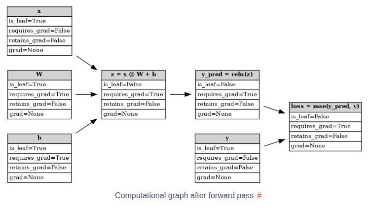
假设存在以下示例网络:
y p r e d = R e L U ( x W + b )
L = M S E ( y p r e d , y )
1 2 3 4 5 6 7 8 9 10 1 , 3 ) 3 , 2 , requires_grad=True ) 1 , 2 , requires_grad=True ) 1 , 2 )
y = f k ( f k − 1 ( … f 1 ( x ) … ) )
∂ y ∂ x = ∂ f k ∂ f k − 1 ⋅ ∂ f k − 1 ∂ f k − 2 ⋅ ⋯ ⋅ ∂ f 1 ∂ x
前向传播之后生成的计算图:
如果一个节点不是由带 requires_grad=True 的张量计算出来的, 那么它就是一个叶子节点, 否则就是非叶子节点. 对于非叶子节点, 其 requires_grad=True 必然是 True, 不然反向传播就无法成功了. 对于叶子节点, 则在初始化时, 需要显式的设置参数 requires_grad=True (默认是 False, 如果初始化时没有设置, 可通过调用 requires_grad_() 方法后补)
retain_grad
在反向传播时,非叶子节点的梯度是会计算的, 但是不会保存在非叶子节点(张量)的 .grad 属性上, 因此它无法使用 .grad 直接访问. 除非显式的设置参数 retain_grad=True
1
2
3
4
5
6
7
8
9
10
11
12
13
14
15
16
17
18
19
20
z = (x @ W) + bNone None print (f"{W.grad=} " )print (f"{b.grad=} " )print (f"{z.grad=} " )print (f"{y_pred.grad=} " )print (f"{loss.grad=} " )
1
2
3
4
5
6
7
W.grad=tensor([[3., 3.],
对于叶子节点, 如果 requires_grad=True, 那么默认是保存梯度的. 此时再额外调用 retain_grad() 属于冗余的操作. 但如果叶子节点的 requires_grad=False 的话, 那么调用 retain_grad() 方法会报错, 因为该节点的梯度不会被计算, 因此自然也无法保存. 所以说, retain_grad() 只在非叶子节点的场景中使用.
主存到显存
主存是分块的, 当 OS 尝试从某个主存块中读取数据却找不到时, 会触发触常, 然后 OS 会从磁盘加载数据到内存中. 同理, 此时如果主存已满, 则 OS 会将部分数据移动到磁盘上, 以便主存能够腾出空间容纳新的数据.
分块的目的是为了能够更充分的利用内存空间, 但是代价是数据的物理内存地址可能不连续. 此时将无法充分发挥 DMA 的效率, 导致将数据复制到 GPU 前需要多一次整理的动作(将数据先复制到缓冲区, 再从缓冲区复制到 GPU), 带来了额外的开锁.
数据在内存中也可以显式设置为固定类型(页锁定, pin_memory), 对于页锁定内在, 它不会被交换到磁盘.
当 OS 加载一个文件时, 它并不会一下子将所有数据都加载到内存中, 而是等到使用时, 如果内存中找不到, 才会触发数据的加载. 当尝试将数据从主存复制到 GPU 的显存时, 由于数据有可能不在主存中, 而是在磁盘中. 为避免等待 IO, 这个复制过程通常是异步的, non_blocking=True
从页锁定的主存中复制数据会更快, 因为数据已经提前加载到内存中了. 同时由于物理地址连续, 可以直接使用 DMA 读取.
数据从主存复制到显存时, CUDA 会自动处理好数据同步问题, 不会出现要读取数据时, 数据却不存在导致报错的情况. 反之, 如果是将数据从显存拷贝到主存, 则需要手工同步一下, 才能保证读取数据前, 数据已经拷贝完成.
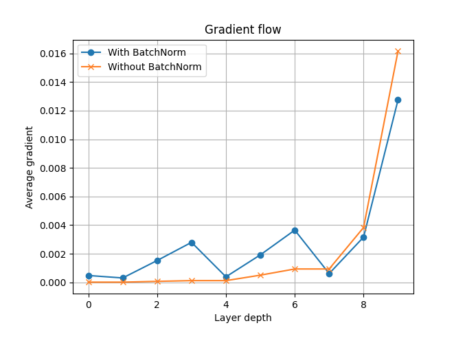
梯度可视化
方便排查处理训练过程中出现的梯度消失或梯度爆炸问题.
示例: 设计两个简单的模型, 一个使用 BatchNorm, 一个没有使用. 并跟踪梯度变化, 以便观察 BatchNorm 能否缓解梯度消失问题.
1
2
3
4
5
6
7
8
9
10
11
12
13
14
15
16
17
18
19
20
21
22
23
24
25
26
27
def fc_layer (in_size, out_size, norm_layer ):"""Return a stack of linear->norm->sigmoid layers""" return nn.Sequential(nn.Linear(in_size, out_size), norm_layer(out_size), nn.Sigmoid())class Net (nn.Module):"""Define a network that has num_layers of linear->norm->sigmoid transformations""" def __init__ (self, in_size=28 *28 , hidden_size=128 , out_size=10 , num_layers=3 , batchnorm=False ):super ().__init__()if batchnorm is False :else :for i in range (num_layers-1 ):self .layers = nn.Sequential(*layers)def forward (self, x ):1 )return self .layers(x)
初始化数据
1 2 3 4 5 6 7 8 9 10 11 12 13 10 , 28 , 28 )10 , (10 , ))True , num_layers=3 )False , num_layers=3 )0.01 , momentum=0.9 )0.01 , momentum=0.9 )
1
2
print (model_bn.layers[0 ])print (model_nobn.layers[0 ])
1
2
3
4
5
6
7
8
9
10
Sequential(
注册钩子
为了能够读取中间状态的数据, 相比使用 retain_grad(), 更推荐的方法是注册反向传播钩子(backward pass hook).
定义钩子:
1
2
3
4
5
6
7
8
9
10
11
12
13
14
15
16
17
18
19
20
21
22
23
24
def hook_forward (module_name, grads, hook_backward ):def hook (module, args, output ):return hookdef hook_backward (module_name, grads ):def hook (grad ):return hookdef get_all_layers (model, hook_forward, hook_backward ):dict ()for name, layer in model.named_modules():if any (layer.children()) is False :return layers, grads
训练并可视化
1
2
3
4
5
6
7
8
9
10
11
12
13
14
15
16
17
18
19
20
21
22
epochs = 10 for epoch in range (epochs):
1
2
3
4
5
6
7
8
9
10
11
12
13
def get_grads (grads ):for idx, (name, grad) in enumerate (grads):if grad is not None :abs ().mean()len (grads) - 1 - idx)return layer_idx, avg_grads
1
2
3
4
5
6
7
8
9
fig, ax = plt.subplots()"With BatchNorm" , marker="o" )"Without BatchNorm" , marker="x" )"Layer depth" )"Average gradient" )"Gradient flow" )True )
分布式训练
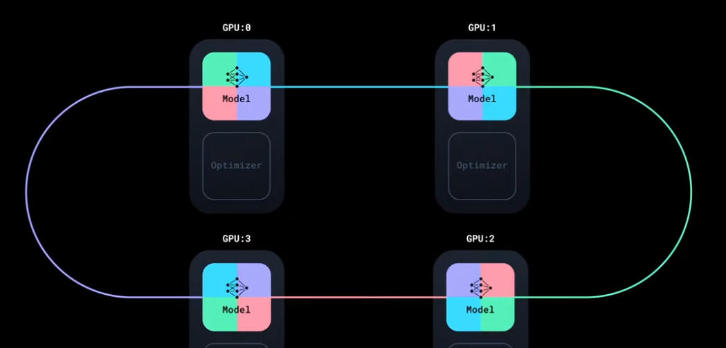
DDP
数据并行, 每张显卡部署相同的模型和优化器. 每张显卡训练的数据不同, 因此在更新参数前, 需要先同步数据, 之后再统一更新参数, 确保更新后的模型参数是每张显卡上面是一样的.
DistributedSampler 可用来确保每张显卡获得的数据不重复
数据的同步是可以并行的, 例如有 4 张显卡, 每次同步 1/4 到另外一张显卡上. 通过使用环状同步, 可以实现同步的并行.
相较早期更简单的 DataParallel, DDP 的性能更好一些, 二者的对比如下:
特性
DataParallel
DistributedDataParallel
开销
更大;模型在每次前向传播时都会被复制并销毁
模型仅复制一次
并行支持
仅支持单机并行
支持扩展到多台机器
性能
速度较慢;在单个进程中使用多线程,会遇到全局解释器锁(GIL)竞争
速度更快(无 GIL 竞争),因为它使用多进程
以下是单 GPU 训练时的代码脚本
1
2
3
4
5
6
7
8
9
10
11
12
13
14
15
16
17
18
19
20
21
22
23
24
25
26
27
28
29
30
31
32
33
34
35
36
37
38
39
40
41
42
43
44
45
46
47
48
49
50
51
52
53
54
55
56
57
58
59
60
61
62
63
64
65
66
67
68
69
70
71
72
73
74
75
76
77
78
79
80
81
82
import torchimport torch.nn.functional as Ffrom torch.utils.data import Dataset, DataLoaderfrom datautils import MyTrainDatasetclass Trainer :def __init__ ( self, model: torch.nn.Module, train_data: DataLoader, optimizer: torch.optim.Optimizer, gpu_id: int , save_every: int , ) -> None :self .gpu_id = gpu_idself .model = model.to(gpu_id)self .train_data = train_dataself .optimizer = optimizerself .save_every = save_everydef _run_batch (self, source, targets ):self .optimizer.zero_grad()self .model(source)self .optimizer.step()def _run_epoch (self, epoch ):len (next (iter (self .train_data))[0 ])print (f"[GPU{self.gpu_id} ] Epoch {epoch} | Batchsize: {b_sz} | Steps: {len (self.train_data)} " )for source, targets in self .train_data:self .gpu_id)self .gpu_id)self ._run_batch(source, targets)def _save_checkpoint (self, epoch ):self .model.state_dict()"checkpoint.pt" print (f"Epoch {epoch} | Training checkpoint saved at {PATH} " )def train (self, max_epochs: int ):for epoch in range (max_epochs):self ._run_epoch(epoch)if epoch % self .save_every == 0 :self ._save_checkpoint(epoch)def load_train_objs ():2048 ) 20 , 1 ) 1e-3 )return train_set, model, optimizerdef prepare_dataloader (dataset: Dataset, batch_size: int ):return DataLoader(True ,True def main (device, total_epochs, save_every, batch_size ):if __name__ == "__main__" :import argparse'simple distributed training job' )'total_epochs' , type =int , help ='Total epochs to train the model' )'save_every' , type =int , help ='How often to save a snapshot' )'--batch_size' , default=32 , type =int , help ='Input batch size on each device (default: 32)' )0
以下是切换到 DDP 模式进行训练的脚本:
1
2
3
4
5
6
7
8
9
10
11
12
13
14
15
16
17
18
19
20
21
22
23
24
25
26
27
28
29
30
31
32
33
34
35
36
37
38
39
40
41
42
43
44
45
46
47
48
49
50
51
52
53
54
55
56
57
58
59
60
61
62
63
64
65
66
67
68
69
70
71
72
73
74
75
76
77
78
79
80
81
82
83
84
85
86
87
88
89
90
91
92
93
94
95
96
97
98
99
100
101
102
103
104
105
106
107
108
import torchimport torch.nn.functional as Ffrom torch.utils.data import Dataset, DataLoaderfrom datautils import MyTrainDatasetimport torch.multiprocessing as mp from torch.utils.data.distributed import DistributedSampler from torch.nn.parallel import DistributedDataParallel as DDP from torch.distributed import init_process_group, destroy_process_group import osdef ddp_setup (rank, world_size ):""" Args: rank: 每个进程的识别代号 world_size: 进程总数 """ "MASTER_ADDR" ] = "localhost" "MASTER_PORT" ] = "12355" "nccl" , rank=rank, world_size=world_size)class Trainer :def __init__ ( self, model: torch.nn.Module, train_data: DataLoader, optimizer: torch.optim.Optimizer, gpu_id: int , save_every: int , ) -> None :self .gpu_id = gpu_idself .model = model.to(gpu_id)self .train_data = train_dataself .optimizer = optimizerself .save_every = save_everyself .model = DDP(model, device_ids=[gpu_id]) def _run_batch (self, source, targets ):self .optimizer.zero_grad()self .model(source)self .optimizer.step()def _run_epoch (self, epoch ):len (next (iter (self .train_data))[0 ])print (f"[GPU{self.gpu_id} ] Epoch {epoch} | Batchsize: {b_sz} | Steps: {len (self.train_data)} " )self .train_data.sampler.set_epoch(epoch) for source, targets in self .train_data:self .gpu_id)self .gpu_id)self ._run_batch(source, targets)def _save_checkpoint (self, epoch ):self .model.module.state_dict()"checkpoint.pt" print (f"Epoch {epoch} | Training checkpoint saved at {PATH} " )def train (self, max_epochs: int ):for epoch in range (max_epochs):self ._run_epoch(epoch)if self .gpu_id == 0 and epoch % self .save_every == 0 :self ._save_checkpoint(epoch)def load_train_objs ():2048 ) 20 , 1 ) 1e-3 )return train_set, model, optimizerdef prepare_dataloader (dataset: Dataset, batch_size: int ):return DataLoader(True ,False , def main (rank: int , world_size: int , save_every: int , total_epochs: int , batch_size: int ):if __name__ == "__main__" :import argparse'simple distributed training job' )'total_epochs' , type =int , help ='Total epochs to train the model' )'save_every' , type =int , help ='How often to save a snapshot' )'--batch_size' , default=32 , type =int , help ='Input batch size on each device (default: 32)' )
异常处理
由于涉及多节点多进程多个 GPU, 训练过程中出现异常的概率会大幅上升. 为避免出现中断导致从头开始训练, 需要引入一个从中断处继续训练的机制. 可使用 pytorch torchrun 提供的 snapshot 功能, 为每轮训练保存快照, 这样当出现中断时, 就可以从快照中快速恢复.
虽然每轮或每几轮会保存 checkpoint 检查点, 但是检查点只包括模型的参数, 没有保存中断前的整个状态, 例如epoch 轮次等. 因此需要在 snapshot 中保存更丰富的信息以便恢复中断时的状态
使用 torchrun 后的几个变化:
无须手动设置 rank, world_size 等环境变量, torchrun 会自动计算
无须手动使用 mp.spawn 孵化多个进程, torchrun 会自动创建多个进程(单节点也可以适用);
当某个进程出现异常导致训练中断后, torchrun 会中断其他所有进程. 再次运行 torchrun 会从中断处继续训练, 损失多少取决于快照保存的时间间隔.
在训练过程中, 如果添加或删除节点, torchrun 会自动在所有节点上重启所有进程, 无需手动干预
引入 snapshot 后, 代码结构大致变成下面这个样子:
1
2
3
4
5
6
7
8
9
10
11
def main ():def train ():for batch in iter (dataset):if should_checkpoint:
以下是引入 torchrun 和 snapshot 后的代码:
1
2
3
4
5
6
7
8
9
10
11
12
13
14
15
16
17
18
19
20
21
22
23
24
25
26
27
28
29
30
31
32
33
34
35
36
37
38
39
40
41
42
43
44
45
46
47
48
49
50
51
52
53
54
55
56
57
58
59
60
61
62
63
64
65
66
67
68
69
70
71
72
73
74
75
76
77
78
79
80
81
82
83
84
85
86
87
88
89
90
91
92
93
94
95
96
97
98
99
100
101
102
103
104
105
106
107
108
109
110
111
112
113
114
115
116
117
import torchimport torch.nn.functional as Ffrom torch.utils.data import Dataset, DataLoaderfrom datautils import MyTrainDatasetimport torch.multiprocessing as mpfrom torch.utils.data.distributed import DistributedSamplerfrom torch.nn.parallel import DistributedDataParallel as DDPfrom torch.distributed import init_process_group, destroy_process_groupimport osdef ddp_setup ():int (os.environ["LOCAL_RANK" ])) "nccl" )class Trainer :def __init__ ( self, model: torch.nn.Module, train_data: DataLoader, optimizer: torch.optim.Optimizer, save_every: int , snapshot_path: str , ) -> None :self .gpu_id = int (os.environ["LOCAL_RANK" ]) self .model = model.to(self .gpu_id)self .train_data = train_dataself .optimizer = optimizerself .save_every = save_everyself .epochs_run = 0 self .snapshot_path = snapshot_pathif os.path.exists(snapshot_path): print ("Loading snapshot" )self ._load_snapshot(snapshot_path)self .model = DDP(self .model, device_ids=[self .gpu_id])def _load_snapshot (self, snapshot_path ):f"cuda:{self.gpu_id} " self .model.load_state_dict(snapshot["MODEL_STATE" ])self .epochs_run = snapshot["EPOCHS_RUN" ]print (f"Resuming training from snapshot at Epoch {self.epochs_run} " )def _run_batch (self, source, targets ):self .optimizer.zero_grad()self .model(source)self .optimizer.step()def _run_epoch (self, epoch ):len (next (iter (self .train_data))[0 ])print (f"[GPU{self.gpu_id} ] Epoch {epoch} | Batchsize: {b_sz} | Steps: {len (self.train_data)} " )self .train_data.sampler.set_epoch(epoch)for source, targets in self .train_data:self .gpu_id)self .gpu_id)self ._run_batch(source, targets)def _save_snapshot (self, epoch ):"MODEL_STATE" : self .model.module.state_dict(),"EPOCHS_RUN" : epoch,self .snapshot_path)print (f"Epoch {epoch} | Training snapshot saved at {self.snapshot_path} " )def train (self, max_epochs: int ):for epoch in range (self .epochs_run, max_epochs):self ._run_epoch(epoch)if self .gpu_id == 0 and epoch % self .save_every == 0 :self ._save_snapshot(epoch)def load_train_objs ():2048 ) 20 , 1 ) 1e-3 )return train_set, model, optimizerdef prepare_dataloader (dataset: Dataset, batch_size: int ):return DataLoader(True ,False ,def main (save_every: int , total_epochs: int , batch_size: int , snapshot_path: str = "snapshot.pt" ):if __name__ == "__main__" :import argparse'simple distributed training job' )'total_epochs' , type =int , help ='Total epochs to train the model' )'save_every' , type =int , help ='How often to save a snapshot' )'--batch_size' , default=32 , type =int , help ='Input batch size on each device (default: 32)' )
1 torchrun --standalone --nproc_per_node=4 multigpu_torchrun.py 50 10
多节点训练
当使用多个节点时, 因为快照只保存在其中一台机器(节点)上, 因此当出现异常导致所有进程重启时, 所有节点都需要从该节点获取快照, 因此有两点很重要, 一是该节点的带宽尽量大一些; 二是确保 TCP 能够连通(注意检查防火墙设置)
由于多节点需要通过网络进行通讯, 其带宽远小于相同节点多个 GPU 之间的通讯带宽, 因此 1 机多卡的训练速度要远大于多机单卡;
有两种方法进行多节点的训练:
在每个节点上面运行相同参数的 torchrun 命令;
创建一个集群, 然后使用一个管理器统一进行调度(例如 slurm);
在单节点场景中, gpu_id 来自 torchrun 设置的 LOCAL_RANK 环境变量. 在多点节场景中, 还需要使用 torchrun 设置的另外一个全局 RANK 环境变量, 以便唯一识别每个 GPU 进程.
当出现异常导致 torchrun 重启所有进程时, 每个进程获得的 LOCAL_RANK 和 RANK 变量可能和之前的不同.
torchrun 支持异构扩展, 即每个节点的 GPU 数量可以不同, 例如有些节点配备 4 个 GPU, 有些配备 2 个GPU
调试时, 可设置环境变量 NCCL_DEBUG=INFO, 这样可以查看详细的日志.
以下是使用多节点训练时的代码变更:
1
2
3
4
5
6
7
8
9
10
11
12
13
14
15
16
17
18
19
20
21
22
23
24
25
26
27
28
29
30
31
32
33
34
35
36
37
38
39
40
41
42
43
44
45
46
47
48
49
50
51
52
53
54
55
56
57
58
59
60
61
62
63
64
65
66
67
68
69
70
71
72
73
74
75
76
77
78
79
80
81
82
83
84
85
86
87
88
89
90
91
92
93
94
95
96
97
98
99
100
101
102
103
104
105
106
107
108
109
110
111
112
import torchimport torch.nn.functional as Ffrom torch.utils.data import Dataset, DataLoaderfrom datautils import MyTrainDatasetimport torch.multiprocessing as mpfrom torch.utils.data.distributed import DistributedSamplerfrom torch.nn.parallel import DistributedDataParallel as DDPfrom torch.distributed import init_process_group, destroy_process_groupimport osdef ddp_setup ():int (os.environ["LOCAL_RANK" ]))"nccl" )class Trainer :def __init__ ( self, model: torch.nn.Module, train_data: DataLoader, optimizer: torch.optim.Optimizer, save_every: int , snapshot_path: str , ) -> None :self .local_rank = int (os.environ["LOCAL_RANK" ]) self .global_rank = int (os.environ["RANK" ]) self .model = model.to(self .local_rank)self .train_data = train_dataself .optimizer = optimizerself .save_every = save_everyself .epochs_run = 0 self .snapshot_path = snapshot_pathif os.path.exists(snapshot_path):print ("Loading snapshot" )self ._load_snapshot(snapshot_path)self .model = DDP(self .model, device_ids=[self .local_rank])def _load_snapshot (self, snapshot_path ):f"cuda:{self.local_rank} " self .model.load_state_dict(snapshot["MODEL_STATE" ])self .epochs_run = snapshot["EPOCHS_RUN" ]print (f"Resuming training from snapshot at Epoch {self.epochs_run} " )def _run_batch (self, source, targets ):self .optimizer.zero_grad()self .model(source)self .optimizer.step()def _run_epoch (self, epoch ):len (next (iter (self .train_data))[0 ])print (f"[GPU{self.global_rank} ] Epoch {epoch} | Batchsize: {b_sz} | Steps: {len (self.train_data)} " ) self .train_data.sampler.set_epoch(epoch)for source, targets in self .train_data:self .local_rank)self .local_rank)self ._run_batch(source, targets)def _save_snapshot (self, epoch ):"MODEL_STATE" : self .model.module.state_dict(),"EPOCHS_RUN" : epoch,self .snapshot_path)print (f"Epoch {epoch} | Training snapshot saved at {self.snapshot_path} " )def train (self, max_epochs: int ):for epoch in range (self .epochs_run, max_epochs):self ._run_epoch(epoch)if self .global_rank == 0 and epoch % self .save_every == 0 :self ._save_snapshot(epoch)def load_train_objs ():2048 ) 20 , 1 ) 1e-3 )return train_set, model, optimizerdef prepare_dataloader (dataset: Dataset, batch_size: int ):return DataLoader(True ,False ,def main (save_every: int , total_epochs: int , batch_size: int , snapshot_path: str = "snapshot.pt" ):if __name__ == "__main__" :import argparse'simple distributed training job' )'total_epochs' , type =int , help ='Total epochs to train the model' )'save_every' , type =int , help ='How often to save a snapshot' )'--batch_size' , default=32 , type =int , help ='Input batch size on each device (default: 32)' )
方案一: 在每台节点上手动单独运行 torchrun 命令
1
2
3
4
5
6
7
8
1
2
3
4
5
6
7
8
方案二: 创建集群, 使用调度器
不同云服务商有不同的创建集群的方法
创建 slurm 脚本
1
2
3
4
5
6
7
8
9
10
11
12
13
14
15
16
17
18
19
20
21
22
23
#!/bin/bash $SLURM_JOB_NODELIST ) )$nodes )${nodes_array[0]} "$head_node " hostname --ip-address)echo Node IP: $head_node_ip export LOGLEVEL=INFO$RANDOM \$head_node_ip :29500 \
运行脚本开始训练
1 sbatch slurm/sbatch_run.sh
可使用 squeue 命令查看任务队列
使用 DDP 模式单机多卡或多机多卡训练 minGPT 的示例
DDP 的实现原理: 给模型的参数注册钩子, 在反向传播时, 将梯度同步到所有进程, 以便所有进程对应的模型的参数梯度值达成最终一致性, 这样各个进程在更新参数后的模型状态能够保持一致.
处理速度差异
不同的进程的计算进度通常有先有后, 在数据同步时, 不同进程之间需要相互等待, 确保所有分片的数据完成同步后, 再进行下一步的计算. 因此需要设置一个足够大的 timeout 值, 避免有些进程在等待的过程中出现超时.
torch.distributed 库中有个 barrier() 方法可用来设置集合点, 确保所有进程到达该集合点后, 再进入下一步. 这样可以避免 A 进程还未保存模型数据, B 进程已经先加载数据并往下计算.
结合模型并行
Model Parallelism, 将模型的不同层放在不同的 GPU 上面, 不同 GPU 组成流水线;
1
2
3
4
5
6
7
8
9
10
11
12
13
14
class ToyMpModel (nn.Module):def __init__ (self, dev0, dev1 ): super (ToyMpModel, self ).__init__()self .dev0 = dev0self .dev1 = dev1self .net1 = torch.nn.Linear(10 , 10 ).to(dev0) self .relu = torch.nn.ReLU()self .net2 = torch.nn.Linear(10 , 5 ).to(dev1) def forward (self, x ):self .dev0) self .relu(self .net1(x))self .dev1) return self .net2(x)
模型并行有几种不同类型:
Tensor Paralelism, 张量并行
Pipeline Paralelism, 流水线并行
Expert Parallelism, 专家并行
不同的 GPU 进程可能收到的 batch 大小不同, 出现不均衡的输入, 会导致不同的进程的迭代次数不一样. 此时某些进程可能提前完成计算, 但其他进程可能还在训练中. 如果让完成计算的进程退出, 会导致后续同步数据时, 其他进程一直处理等待的状态, 最终造成死锁.
为避免这个问题 torch.distributed.algorithms.join 库中引入了 Join 上下文管理器. 当某些进程提前完成数据的计算后, 会进入 join 模式. 在这个模式下, 该进程不会提前退出, 而是会假装仍在工作, 会继续参与数据同步的工作, 只是它发的梯度数据是零, 同时在 step 时也不会更新模型的参数. 直到所有进程都完成计算后, 整个上下文才会终止.
1
2
3
4
5
6
7
8
9
10
11
12
13
14
15
16
17
18
19
20
21
22
23
24
25
26
27
28
29
30
31
32
33
34
import osimport torchimport torch.distributed as distimport torch.multiprocessing as mpfrom torch.distributed.algorithms.join import Joinfrom torch.nn.parallel import DistributedDataParallel as DDP"nccl" 2 5 def worker (rank ):'MASTER_ADDR' ] = 'localhost' 'MASTER_PORT' ] = '29500' 1 , 1 ).to(rank), device_ids=[rank])1 ]).float () for _ in range (NUM_INPUTS + rank)]0 with Join([model]): for input in inputs:1 input ).sum ()print (f"Rank {rank} has exhausted all {num_inputs} of its inputs!" )def main ():True )if __name__ == "__main__" :
Join 还可以同时管理多个类, 例如 ZeroRedundancyOptimizer, 示例如下:
ZeroRedundancyOptimizer 用来给优化器状态进行分片, 这样优化器的数据也可以像梯度一样是分布式的, 好处是可以减少单个 GPU 的内存占用, 等实际需要使用时, 多个 GPU 之间再进行同步即可. 缺点是需要付出一点数据同步的时间. 以时间换空间, 是否使用要看用哪种优化器, 有些优化器的状态占内存较多, 例如 Adam. 有些则没有;
1
2
3
4
5
6
7
8
9
10
11
12
13
14
15
16
17
18
19
20
21
22
from torch.distributed.optim import ZeroRedundancyOptimizer as ZeROfrom torch.optim import Adamdef worker (rank ):'MASTER_ADDR' ] = 'localhost' 'MASTER_PORT' ] = '29500' 1 , 1 ).to(rank), device_ids=[rank])0.01 ) 1 ]).float () for _ in range (NUM_INPUTS + rank)]0 with Join([model, optim]): for input in inputs:1 input ).sum ()print (f"Rank {rank} has exhausted all {num_inputs} of its inputs!" )
Join 支持传入一些参数
1 2 3 4 with Join([model, optim], divide_by_initial_world_size=False ):for input in inputs:
FSDP2
Fully Sharded Data Parallel, 全分片数据并行. DDP 只是训练数据分片, FSDP 则更进一步, 连模型参数, 优化器状态都进行分片, 这样做的好处是可以减少单个 GPU 的内存容量要求.
由于 FSDP 将模型的参数也分片了, 因此相比 DDP, 它不仅要同步梯度, 还多了一个同步参数的动作. 即每个 GPU 需要先all-gather 动态的收集其他 GPU 上面的参数, 基于完整的模型参数计算出结果后, 再释放掉内存, 只保留自己所负责的那部分参数. 所以从结果上来看, 每个 GPU 上面的模型参数好像是完整的, 但实际上这种完整是一种临时拼凑的状态,是一种逻辑上的完整,而不是物理上的完整. 计算结束后, 实际保存的仍然只是一个参数分片.
FSDP 或许可视为一种更加激进的分片策略, 通过极致的以时间换空间, 进一步压榨 GPU 显存
模型初始化
1
2
3
4
5
6
7
8
9
10
11
12
13
14
15
16
17
18
from torch.distributed.fsdp import fully_shard, FSDPModulefor layer in model.layers:assert isinstance (model, Transformer)assert isinstance (model, FSDPModule)print (model)
fully_shard 会将模型的参数由 Tensor 转成 DTensor 类型(一种数据抽象), 用来表示它是做了分片的参数. DTensor 有助于简化各项操作的逻辑, 减少手动处理这些分片数据的同步工作.
FSDP2 在参数的第一个维度上进行分片, 因此第一维的数量需要是 world size 的倍数, 否则无法均匀分片. 此时 FSDP 默认会报错.
由于 FSDP2 模式下参数是分片的, 因此在保存模型时, 可以借助 DCP(Distributed Checkpointing)实现分布式保存. 每个 GPU 进程只保存自己的那部分参数, 这样可以减少通讯成本. 后续加载参数时, 每个 GPU 也可以只加载自己负责的那部分参数.
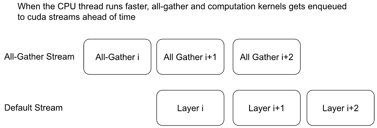
前向/后向预取
由于模型参数是分片, 计算前需要实时 all-gather 聚合, 这样就涉及了通信的时间. 理想情况下让计算和通信同时进行, 这样计算的时候,不用等待通信. 有两种实现的方案:
隐式预取: 在计算当前层的时候, 后台自动偷偷 all-gather 预取下一个 layer 或 block 所需的参数.
显式预取: 手动控制什么时候预取参数, 好处是非常灵活, 一般有以下几种使用场景:
隐式只预取一层, 显式则可以预取多层, 好处是减少等待的发生, 缺点是占用多一些内存空间;
预热: 在调用 model(x) 之前先预取, 这样调用 model 后直接开算, 不用等待;
CPU 工作负载过高, 没有及时发出预取指令, 造成空闲等待, 因此只能手动完成;
以下是隐式预取的图示:
以下是显式预取的代码示例:
1
2
3
4
5
6
7
8
9
10
11
12
13
14
15
16
17
18
19
20
21
22
23
24
25
num_to_forward_prefetch = 2 for i, layer in enumerate (model.layers):if i >= len (model.layers) - num_to_forward_prefetch:break for j in range (1 , num_to_forward_prefetch + 1 )2 for i, layer in enumerate (model.layers):if i < num_to_backward_prefetch:continue for j in range (1 , num_to_backward_prefetch + 1 )for _ in range (epochs):0 , vocab_size, (batch_size, seq_len), device=device)sum ()
开启混合精度
FSDP2 支持灵活的混合精度策略, 以便提高训练的速度. 典型用法示例:
在前向和后向传播将默认的 float32 转成 bfloat16 类型, 这样可以节省显存占用;
做梯度聚合时, 将 bfloat16 类型转回 float32, 以便提高梯度计算的精度, 避免误差可能带来的发散;
1
2
3
4
5
6
7
8
9
10
11
12
13
14
15
16
17
18
19
20
21
22
23
24
25
26
27
model = Transformer(model_args)"mp_policy" : MixedPrecisionPolicy( for layer in model.layers:for param in model.parameters():assert param.dtype == torch.float32for param in model.parameters(recurse=False ):assert param.dtype == torch.bfloat161e-2 )
梯度裁剪与基于 DTensor 的优化器
在 full_shard 模型后, 再初始化优化器, 以便优化器能够正确跟踪分布在不同 GPU 上面的参数分片.
参数分片后的包装类型是 DTensor, 它默认支持梯度裁剪. 梯度裁剪涉及计算范数, 此时需要先聚合梯度. DTensor 会自动拦截各种张量 Tensor 的正常操作, 然后在需要时会自动完成通信聚合的相关工作, 对用户来说是透明的.
TP
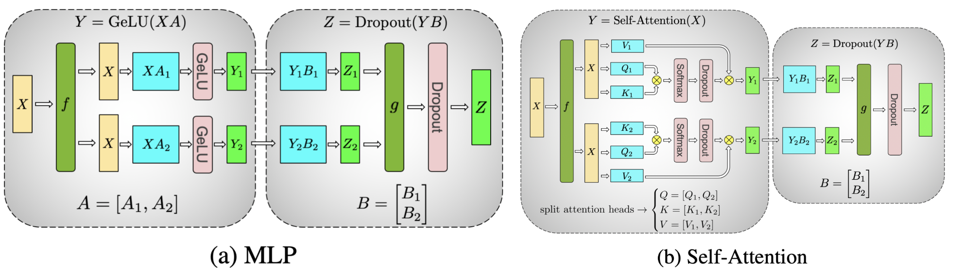
工作原理
对张量进行拆分计算的示意图, 例如 MLP 和自注意力两种计算场景:
TP 的工作原理主要由三部分构成:
静态分片
模型初始化时, TP 为模型的每一层选择不同的并行策略(按行或按列)
调用 parallelize_module 将模型转换为并行版本;
将普通张量 Tensor 转换为支持并行的 DTensor 张量(自动处理跨设备的通信)
动态通信
all-reduce
all-gather
reduce-scatter
局部计算: 每个 GPU 只负责计算自己负责的那部分分片数据;
使用场景
虽然 FSDP 已经能够实现数据并行, 也能够对模型参数进行切片, 但它仍然面临一些瓶颈:
当 GPU 数量变多时, 通信成本变成瓶颈;
每个 GPU 的 batch size 最小为 1, 过多的 GPU 导致总体 batch size 非常大. 但过大的 batch size 可能导致收敛不稳定;
较小的 batth size 有可能无法满足 GPU 的形状规整要求(例如维度是 8, 16, 32 的倍数), 导致浮点运算的效率不高;
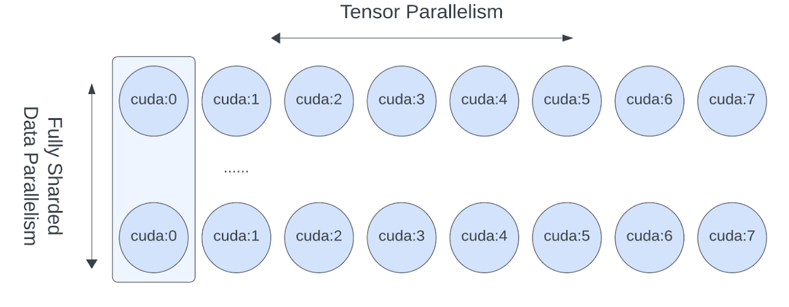
TP/SP 刚好可以用来解决以上问题:
在节点间使用 FSDP, 单节点内部的多 GPU 之间使用 TP, 这样可以显著减少通信成本. 例如一机八卡, 那么节点间的通信成本可以除以 8 倍;相当于 FSDP 是以节点进行切片, 而不是以 GPU 进行切片;
张量支持切片后, GPU 的 batch size 就可以小于 1 了, 二者实现了解耦;
张量切片有助于满足 GPU 浮点运算对矩阵形状的规整要求;
问题
解决方案
效果
FSDP 在超大规模 GPU 下通信开销大
节点内用 TP/SP,节点间用 FSDP
减少 FSDP 通信域,降低延迟
数据并行受批大小限制
引入 TP/SP 解耦 GPU 数与批大小
可继续增加 GPU 而不破坏收敛
小 batch 导致计算效率低
TP/SP 优化矩阵形状
提高 FLOPS 利用率
使用方法
1 2 3 4 from torch.distributed.device_mesh import init_device_mesh"cuda" , (8 ,))
如何实施张量并行, 取决于模型某一层如何进行计算, 因此要视具体情况而定, 举例如下:
1 2 3 def forward (self, x ):return self .w2(F.silu(self .w1(x)) * self .w3(x))
w1 和 w3 是两个线性层, 是可以并行的矩阵乘法运算, w2 同样是线性层, 基于前二者的逐元素相乘的结果再做矩阵乘法;
第1步: w1 和 w3 是单独对输入 x 做矩阵乘法, 因此二者可以按列切片, 这样每个 GPU 只需计算自己负责的那一部分列即可;x 则需要完整的广播到所有 GPU, 没有切片;
第2步: w1 和 w3 是逐元素相乘, 因此前面的计算结果仍然可以在 GPU 内部做局部计算, 无须和其他 GPU 进行通信;
第3步: w2 是矩阵乘法, 可将 w2 按行切分, 每个 GPU 单独计算出一部分结果, 最后通过 all reduce 聚合成完整的结果;
1 2 3 4 5 6 7 8 from torch.distributed.tensor.parallel import ColwiseParallel, RowwiseParallel, parallelize_module"feed_foward.w1" : ColwiseParallel(),"feed_forward.w2" : RowwiseParallel(),"feed_forward.w3" : ColwiseParallel(),
组件
并行方式
输入布局
输出布局
是否需要通信
w1, w3Column-wise
Replicated
Sharded
否(各自独立计算)
w1(x) * w3(x)Element-wise
Sharded
Sharded
否(同设备上直接相乘)
w2Row-wise
Sharded
Replicated(经 all-reduce)
是(最后一次 all-reduce)
以上示例是 feed_forward 层, 对于 Transformer 模块中的 self attention 注意力层, 并行策略大概类似:
1 2 3 4 5 6 7 8 9 10 11 12 13 layer_tp_plan = {"attention.wq" : ColwiseParallel(use_local_output=False ),"attention.wk" : ColwiseParallel(use_local_output=False ),"attention.wv" : ColwiseParallel(use_local_output=False ),"attention.wo" : RowwiseParallel(),"feed_forward.w1" : ColwiseParallel(),"feed_forward.w2" : RowwiseParallel(),"feed_forward.w3" : ColwiseParallel(),
使用 parallel_module 函数将 transformer block 转换成张量并行模式
1 2 3 4 5 6 7 8 for layer_id, transformer_block in enumerate (model.layers):
对于模型头部的 Embedding 层和尾部的 Linear 层, 采用类似的张量并行策略
1 2 3 4 5 6 7 8 9 10 11 12 13 14 model = parallelize_module("tok_embeddings" : RowwiseParallel("output" : ColwiseParallel(
用于归一化层
SP(sequence parallel, 序列并行), 是 TP 张量并行的一个变体. TP 是对权重进行切分, 比如按矩阵的行或列. 而 SP 则更进一步, 对输入序列的长度进行切分. 它主要用于 LayerNorm 或者 RMSNorm 等归一化层中, 将一个长序列切分成多个片段, 每个 GPU 负责处理其中一个片段. 目的是为了减少激活值所占用的内存. 因为激活值会随着输入序列的长度和批量大小呈线性增长.
SP: Shard(1), 在第1维(seq维)进行切分, [batch, seq_len, hidden_dim] 变成 [batch, seq_len / N, hidden_dim]
RMSNorm 或 LayerNorm 等归一化层是在 hiddem_dim 维度上做归一化, 与 sequence 维度无关, 因此归一化层很适合用来分片, 不同分片之间无需通信. 而 Attention 或 FeedForward 则不适合用来做 SP, 因为它们的矩阵需要完整的行或列, SP 后会带来很大的通信成本.
代码示例如下:
1 2 3 4 5 6 7 8 9 10 11 12 13 14 15 16 17 18 19 20 21 22 23 24 25 from torch.distributed.tensor.parallel import ("attention_norm" : SequenceParallel(), "attention" : PrepareModuleInput(1 ), Replicate()), "attention.wq" : ColwiseParallel(use_local_output=False ),"attention.wk" : ColwiseParallel(use_local_output=False ),"attention.wv" : ColwiseParallel(use_local_output=False ),"attention.wo" : RowwiseParallel(output_layouts=Shard(1 )),"ffn_norm" : SequenceParallel(), "feed_forward" : PrepareModuleInput(1 ),), "feed_forward.w1" : ColwiseParallel(),"feed_forward.w2" : RowwiseParallel(output_layouts=Shard(1 )),"feed_forward.w3" : ColwiseParallel(),
1 2 3 4 5 6 7 8 9 10 11 12 13 14 15 16 "tok_embeddings" : RowwiseParallel(嵌入层1 ), "norm" : SequenceParallel(),"output" : ColwiseParallel(1 ),
损失并行
如果 vocal_size 已经是分片的, 那么在计算损失时, 每个 GPU 也可先做自己负责的 logits 的局部交叉熵损失计算, 之后再 reduce 得到最终的 loss;
1 2 3 4 with loss_parallel():
1 2 3 4 5 6 7 8 9 10 11 12 13 14 15 16 model = parallelize_module("tok_embeddings" : RowwiseParallel(1 ),"norm" : SequenceParallel(),"output" : ColwiseParallel(1 ),False ,
结合 FSDP
FSDP 负责节点间的切片, TP 负责单节点多个 GPU 间的切片
以上切分方式可通过设置 DeviceMesh 的参数来实现
1 2 3 4 5 6 7 8 9 10 11 12 13 14 15 16 17 from torch.distributed.device_mesh import init_device_meshfrom torch.distributed.tensor.parallel import ColwiseParallel, RowwiseParallel, parallelize_modulefrom torch.distributed.fsdp import fully_shard"cuda" , (8 , 8 ))"tp" ] "dp" ]
使用 FSDP + TP 的代码示例
DeviceMesh
DeviceMesh 是用来管理进程组的一个高级抽象, 简化手动管理这些进程的工作, 例如给每个进程分配 rank id
1 2 3 4 5 6 7 8 from torch.distributed.device_mesh import init_device_mesh"cuda" , (2 , 4 ), mesh_dim_names=("replicate" , "shard" ))"replicate" )"shard" )
HSDP
HSDP, Hybrid Sharding Data Paralelism, 混合数据并行, 单节点内部使用 FSDP, 多节点之间使用 DDP
1 2 3 4 5 6 7 8 9 10 11 12 13 14 15 16 17 18 19 20 21 22 23 import torchimport torch.nn as nnfrom torch.distributed.device_mesh import init_device_meshfrom torch.distributed.fsdp import fully_shard as FSDPclass ToyModel (nn.Module):def __init__ (self ):super (ToyModel, self ).__init__()self .net1 = nn.Linear(10 , 10 )self .relu = nn.ReLU()self .net2 = nn.Linear(10 , 5 )def forward (self, x ):return self .net2(self .relu(self .net1(x)))"cuda" , (2 , 4 ), mesh_dim_names=("dp_replicate" , "dp_shard" ))
自定义并行方案
对于复杂的自定义并行方案, DeviceMesh 支持从网格中提取子网格, 进行一些自定义的操作
1 2 3 4 5 6 7 8 9 10 11 12 13 from torch.distributed.device_mesh import init_device_mesh"cuda" , (2 , 2 , 2 ), mesh_dim_names=("replicate" , "shard" , "tp" ))"replicate" , "shard" ]"tp" ]"replicate" ].get_group()"shard" ].get_group()
PP
Pipeline Paralism, 流水线并行. 当模型太大, 无法放入单个 GPU 时, 可考虑使用 PP 并行模式. 将模型按层或模块拆分为多个 stage, 每个 GPU 负责一部分 stage;同时将一个 batch 的数据, 也拆分成多个小的 micro-batch, 逐个输入流水线.
micro-batch 的好处是小步快跑,这样有助于让多个 stage 同时跑起来;如果没有拆分, 则后面的 stage 需要等待前面的 stage 处理完;尽管如此, 启动和结束时出现一个小的等待窗口仍然是不可避免的, 称为 bubble;
执行顺序如下(时间步 t1, t2, …):
时间
S1(设备0)
S2(设备1)
t1
M1 前向
——
t2
M2 前向
M1 前向 + 反向
t3
M3 前向
M2 前向 + 反向
t4
M4 前向
M3 前向 + 反向
t5
——
M4 前向 + 反向